Nobody Understands Probability
Published:
The goal of this post is to give an overview of Bayesian statistics as well as to correct errors about probability that even mathematically sophisticated people commonly make. Hopefully by the end of this post I will convince you that you don’t actually understand probability theory as well as you think, and that probability itself is something worth thinking about.
I will try to make this post somewhat shorter than the previous posts. As a result, this will be only the first of several posts on probability. Even though this post will be shorter, I will summarize its organization below:
- Bayes’ theorem: the fundamentals of conditional probability
- modeling your sources: how not to calculate conditional probabilities; the difference between “you are given X” and “you are given that you are given X”
- how to build models: examples using toy problems
- probabilities are statements about your beliefs (not the world)
- re-evaluating a standard statistical test
I bolded the section on models because I think it is very important, so I hope that bolding it will make you more likely to read it.
Also, I should note that when I say that nobody understands probability, I don’t mean it in the sense that most people are bad at combinatorics. Indeed, I expect that most of the readers of this blog are quite proficient at combinatorics, and that many of them even have sophisticated mathematical definitions of probability. Rather I would say that actually using probability theory in practice is non-trivial. This is partially because there are some subtleties (or at least, I have found myself tripped up by certain points, and did not realize this until much later). It is also because whenever you use probability theory in practice, you end up employing various heuristics, and it’s not clear which ones are the “right” ones.
If you disagree with me, and think that everything about probability is trivial, then I challenge you to come up with a probability-theoretic explanation of the following phenomenon:
Suppose that you have never played a sport before, and you play soccer, and enjoy it. Now suppose instead that you have never played a sport before, and play soccer, and hate it. In the first case, you will think yourself more likely to enjoy other sports in the future, relative to in the second case. Why is this?
Or if you disagree with the premises of the above scenario, simply “If X and Y belong to the same category C, why is it that in certain cases we think it more likely that Y will have attribute A upon observing that X has attribute A?”
Bayes’ Theorem
Bayes’ theorem is a fundamental result about conditional probability. It says the following:
$p(A \mid B) = \frac{p(B \mid A)p(A)}{p(B)}$
Here $A$ and $B$ are two events, and $p(A \mid B)$ means the probability of $A$ conditioned on $B$. In other words, if we already know that $B$ occurred, what is the probability of $A$? The above theorem is quite easy to prove, using the fact that $p(A \cap B) = p(A \mid B)p(B)$, and thus also equals $p(B \mid A)p(A)$, so that $p(A \mid B)p(B) = p(B \mid A)p(A)$, which implies Bayes’ theorem. So, why is it useful, and how do we use it?
One example is the following famous problem: A doctor has a test for a disease that is 99% accurate. In other words, it has a 1% chance of telling you that you have a disease even if you don’t, and it has a 1% chance of telling you that you don’t have a disease even if you do. Now suppose that the disease that this tests for is extremely rare, and only affects 1 in 1,000,000 people. If the doctor performs the test on you, and it comes up positive, how likely are you to have the disease?
The answer is close to $10^{-4}$, since it is roughly $10^4$ times as likely for the test to come up positive due to an error in the test relative to you actually having the disease. To actually compute this with Bayes’ rule, you can say
| p(Disease | Test is positive) = p(Test is positive | Disease)p(Disease)/p(Test is positive), |
which comes out to $\frac{0.99 \cdot 10^{-6}}{0.01 \cdot (1-10^{-6}) + 0.99 \cdot 10^{-6}},$ which is quite close to $10^{-4}$.
In general, we can use Bayes’ law to test hypotheses:
| p(Hypothesis | Data) = p(Data | Hypothesis) p(Hypothesis) / p(Data) |
Let’s consider each of these terms separately:
p(Hypothesis Data) — the weight we assign to a given hypothesis being correct under our observed data p(Data Hypothesis) — the likelihood of seeing the data we saw under our hypothesis; note that this should be quite easy to compute. If it isn’t, then we haven’t yet fully specified our hypothesis. - p(Hypothesis) — the prior weight we give to our hypothesis. This is subjective, but should intuitively be informed by the consideration that “simpler hypotheses are better”.
- p(Data) — how likely we are to see the data in the first place. This is quite hard to compute, as it involves considering all possible hypotheses, how likely each of those hypotheses is to be correct, and how likely the data is to occur under each hypothesis.
| So, we have an expression for p(Hypothesis | Data), one of which is easy to compute, the other of which can be chosen subjectively, and the last of which is hard to compute. How do we get around the fact that p(Data) is hard to compute? Note that p(Data) is independent of which hypothesis we are testing, so Bayes’ theorem actually gives us a very good way for comparing the relative merits of two hypotheses: |
| p(Hypothesis 1 | Data) / p(Hypothesis 2 | Data) = [p(Data | Hypothesis 1) / p(Data | Hypothesis 2)] $\times$ p(Hypothesis 1) / p(Hypothesis 2) |
Let’s consider the following toy example. There is a stream of digits going past us, too fast for us to tell what the numbers are. But we are allowed to push a button that will stop the stream and allow us to see a single number (whichever one is currently in front of us). We push this button three times, and see the numbers 3, 5, and 3. How many different numbers would we estimate are in the stream?
For simplicity, we will make the (somewhat unnatural) assumption that each number between 0 and 9 is selected to be in the stream with probability 0.5, and that each digit in the stream is chosen uniformly from the set of selected numbers. It is worth noting now that making this assumption, rather than some other assumption, will change our final answer.
Now under this assumption, what is the probability, say, of there being exactly 2 numbers (3 and 5) in the stream? By Bayes’ theorem, we have
$p(\{3,5\} \mid (3,5,3)) \propto p((3,5,3) \mid \{3,5\}) p(\{3,5\}) = \left(\frac{1}{2}\right)^3 \left(\frac{1}{2}\right)^{10}.$
Here $\propto$ means “is proportional to”.
What about the probability of there being 3 numbers (3, 5, and some other number)? For any given other number, this would be
$p(\{3,5,x\} \mid (3,5,3)) \propto p((3,5,3) \mid \{3,5,x\}) p(\{3,5,x\}) = \left(\frac{1}{3}\right)^3 \left(\frac{1}{2}\right)^{10}.$
However, there are 8 possibilities for $x$ above, all of which correspond to disjoint scenarios, so the probability of there being 3 numbers is proportional to $9 \left(\frac{1}{3}\right)^3 \left(\frac{1}{2}\right)^{10}$. If we compare this to the probability of there being 2 numbers, we get
| $p(2 \text{ numbers} | (3,5,3)) / p(3 \text{ numbers} | (3,5,3)) = 3/8$. |
Even though we have only seen two numbers in our first three samples, we still think it is more likely that there are 3 numbers than 2, just because the prior likelihood of there being 3 numbers is so much higher. However, suppose that we made 6 draws, and they were 3,5,3,3,3,5. Then we would get
| $p(2 \text{ numbers} | (3,5,3,3,5)) / p(3 \text{ numbers} | (3,5,3,3,5)) = (1/2)^6 / [9 \times (1/3)^6] = 81/64$. |
Now we find it more likely that there are only 2 numbers. This is what tends to happen in general with Bayes’ rule — over time, more restrictive hypotheses become exponentially more likely than less restrictive hypotheses, provided that they correctly explain the data. Put another way, hypotheses that concentrate probability density towards the actual observed events will do best in the long run. This is a nice feature of Bayes’ rule because it means that, even if the prior you choose is not perfect, you can still arrive at the “correct” hypothesis through enough observations (provided that the hypothesis is among the set of hypotheses you consider).
I will use Bayes’ rule extensively through the rest of this post and the next few posts, so you should make sure that you understand it. If something is unclear, post a comment and I will try to explain in more detail.
Model Your Sources
An important distinction that I think most people don’t think about is the difference between experiments you perform, and experiments you observe. To illustrate what I mean by this, I would point to the difference between biology and particle physics – where scientists set out to test a hypothesis by creating an experiment specifically designed to do so — and astrophysics and economics, where many “experiments” come from seeking out existing phenomena that can help evaluate a hypothesis.
To illustrate why one might need to be careful in the latter case, consider empirical estimates of average long-term GDP growth rate. How would one do this? Since it would be inefficient to wait around for the next 10 years and record the data of all currently existing countries, instead we go back and look at countries that kept records allowing us to compute GDP. But in this case we are only sampling from countries that kept such records, which implies a stable government as well as a reasonable degree of economics expertise within that government. So such a study almost certainly overestimates the actual average growth rate.
Or as another example, we can argue that a scientist is more likely to try to publish a paper if it doesn’t agree with prevalent theories than if it does, so looking merely at the proportion of papers that lend support to or take support away from a theory (even if weighted by the convincingness of each paper) is probably not a good way to determine the validity of a theory.
So why are we safer in the case that we forcibly gather our own data? By gathering our own data, we understand much better (although still not perfectly) the way in which it was constructed, and so there is less room for confounding parameters. In general, we would like it to be the case that the likelihood of observing something that we want to observe does not depend on anything else that we care about — or at the very least, we would like it to depend in a well-defined way.
Let’s consider an example. Suppose that a man comes up to you and says “I have two children. At least one of them is a boy.” What is the probability that they are both boys?
The standard way to solve this is as follows: Assuming that male and female children are equally likely, there is a $\frac{1}{4}$ chance of two girls or two boys, and a $\frac{1}{2}$ chance of having one girl and one boy. Now by Bayes’ theorem,
| p(Two boys | At least one boy) = p(At least one boy | Two boys) $\times$ p(Two boys) / p(At least one boy) = 1 $\times$ (1/4) / (1/2+1/4) = 1/3. |
So the answer should be 1/3 (if you did math contests in high school, this problem should look quite familiar). However, the answer is not, in fact, 1/3. Why is this? We were given that the man had at least one boy, and we just computed the probability that the man had at two boys given that he had at least one boy using Bayes’ theorem. So what’s up? Is Bayes’ theorem wrong?
No, the answer comes from an unfortunate namespace collision in the word “given”. The man “gave” us the information that he has at least one male child. By this we mean that he asserted the statement “I have at least one male child.” Now our issue is when we confuse this with being “given” that the man has at least one male child, in the sense that we should restrict to the set of universes in which the man has at least one male child. This is a very different statement than the previous one. For instance, it rules out universes where the man has two girls, but is lying to us.
Even if we decide to ignore the possibility that the man is lying, we should note that most universes where the man has at least one son don’t even involve him informing us of this fact, and so it may be the case that proportionally more universes where the man has two boys involve him telling us “I have at least one male child”, relative to the proportion of such universes where the man has one boy and one girl. In this case the probability that he has two boys would end up being greater than 1/3.
The most accurate way to parse this scenario would be to say that we are given (restricted to the set of possible universes) that we are given (the man told us that) that the man has at least one male child. The correct way to apply Bayes’ rule in this case is
| p(X has two boys | X says he has $\geq$ 1 boy) = p(X says he has $\geq$ 1 boy | X has two boys) $\times$ p(X has two boys) / p(X says he has $\geq $1 boy) |
If we further assume that the man is not lying, and that male and female children are equally likely and uncorrelated, then we get
| p(X has two boys | X says he has $\geq$ 1 boy) = [p(X says he has $\geq$ 1 boy | X has two boys) $\times$ 1/4]/[p(X says he has $\geq$ 1 boy | X has two boys) $\times$ 1/4 + p(X says he has $\geq$ 1 boy | X has one boy) $\times$ 1/2] |
So if we think that the man is $\alpha$ times more likely to tell us that he has at least one boy when he has two boys, then
| p(X has two boys | X says he has $\geq$ 1 boy) = $\frac{\alpha}{\alpha+2}$. |
Now this means that if we want to claim that the probability that the man has two boys is $\frac{1}{3}$, what we are really claiming is that he is equally likely to inform us that he has at least one boy, in all situations where it is true, independent of the actual gender distribution of his children.
I would argue that this is quite unlikely, as if he has a boy and a girl, then he could equally well have told us that he has at least one girl, whereas he couldn’t tell us that if he has only boys. So I would personally put $\alpha$ closer to 2, which yields an answer of $\frac{1}{2}$. On the other hand, situations where someone walks up to me and tells me strange facts about the gender distribution of their children are, well, strange. So I would also have to take into account the likely psychology of such a person, which would end up changing my estimate of $\alpha$.
The whole point here is that, because we were an observer receiving information, rather than an experimenter acquiring information, there are all sorts of confounding factors that are difficult to estimate, making it difficult to get a good probability estimate (more on that later). That doesn’t mean that we should give up and blindly guess $\frac{1}{3}$, though — it might feel like doing so gets away without making unwarranted assumptions, but it in fact implicitly makes the assumption that $\alpha = 1$, which as discussed above is almost certainly unwarranted.
What it does mean, though, is that, as scientists, we should try to avoid situations like the one above where there are lots of confounding factors between what we care about and our observations. In particular, we should avoid uncertainties in the source of our information by collecting the information ourselves.
I should note that, even when we construct our own experiments, we should still model the source of our information. But doing so is often much easier. In fact, if we wanted to be particularly pedantic, we really need to restrict to the set of universes in which our personal consciousness receives a particular set of stimuli, but that set of stimuli has almost perfect correlation with photons hitting our eyes, which has almost perfect correlation with the set of objects in front of us, so going to such lengths is rarely necessary — we can usually stop at the level of our personal observations, as long as we remember where they come from.
How to Build Models
Now that I’ve told you that you need to model your information sources, you perhaps care about how to do said modeling. Actually, constructing probabilistic models is an extremely important skill, so even if you ignore the rest of this post, I recommend paying attention to this section.
This section will have the following examples:
- Determining if a coin is fair
- Finding clusters
Determining if a Coin is Fair
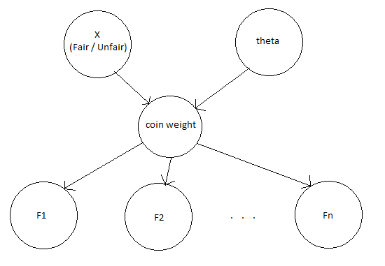
Suppose that you have occasion to observe a coin being flipped (or better yet, you flip it yourself). You do this several times and observe a particular sequence of heads and tails. If you see all heads or all tails, you will probably think the coin is unfair. If you see roughly half heads and half tails, you will probably think the coin is fair. But how do we quantify such a calculation? And what if there are noticeably many more heads than tails, but not so many as to make the coin obviously unfair?
We’ll solve this problem by building up a model in parts. First, there is the thing we care about, namely whether the coin is fair or unfair. So we will construct a random variable X that can take the values Fair and Unfair. Then p(X = Fair) is the probability we assign to a generic coin being fair, and p(X = Unfair) is the probability we assign to a generic coin being unfair.
| Now supposing the coin is fair, what do we expect? We expect each flip of the coin to be independent, and have a $\frac{1}{2}$ probability of coming up heads. So if we let F1, F2, …, Fn be the flips of the coin, then p(Fi = Heads | X = Fair) = 0.5. |
| What if the coin is unfair? Let’s go ahead and blindly assume that the flips will still be independent, and furthermore that each possible weight of the coin is equally likely (this is unrealistic, as weights near 0 or 1 are much more likely than weights near 0.5). Then we have to have an extra variable $\theta$, the probability that the unfair coin comes up heads. So we have p(Unfair coin weight = $\theta$) = 1. Note that this is a probability density, not an actual probability (as opposed to p(Fi = Heads | X = Fair), which was a probability). |
| Continuing, if F1, F2, …, Fn are the flips of the coin, then p(Fi = Heads | X = Fair, Weight = $\theta$) = $\theta$. |
Now we’ve set up a model for this problem. How do we actually calculate a posterior probability of the coin being fair for a given sequence of heads and tails? (A posterior probability is just the technical term for the conditional probability of a hypothesis given a set of data; this is to distinguish it from the prior probability of the hypothesis before seeing any data.)
Well, we’ll still just use Bayes’ rule:
| p(Fair | F1, …, Fn) $\propto$ p(F1, …, Fn | Fair) p(Fair) = $\left(\frac{1}{2}\right)^n$ p(Fair) |
| p(Unfair | F1, …, Fn) $\propto$ p(F1, …, Fn | Unfair) p(Unfair) = $\int_{0}^{1} \theta^{H}(1-\theta)^{T} d\theta$ p(Unfair) |
Here H is the number of heads and T is the number of tails. In this case we can fortunately actually compute the integral in question and see that it is equal to $\frac{H!T!}{(H+T+1)!}$. So we get that
| p(Fair | F1, …, Fn) / p(Unfair | F1, …, Fn) = p(Fair)/p(Unfair) $\times$ $\frac{(H+T+1)!}{2^n H!T!}$. |
It is often useful to draw a diagram of our model to help keep track of it:
Now suppose that we, being specialists in determining if coins are fair, have been called in to study a large collection of coins. We get to one of the coins in the collection, flip it several times, and observe the following sequence of heads and tails:
HHHHTTTHHTTT
Since there are an equal number of heads and tails, our previous analysis will certainly conclude that the coin is fair, but its behavior does seem rather suspicious. In particular, different flips don’t look like they are really independent, so perhaps our previous model is wrong. Maybe the right model is one where the next coin value is usually the same as the previous coin value, but flips with some probability. Now we have a new value of X, which we’ll call Weird, and a parameter $\phi$ (basically the same as $\theta$) that tells us how likely a weird coin is to have a given probability of switching. We’ll again give $\phi$ a uniform distribution over [0,1], so p(Switching probability of weird coin = $\phi$) = 1.
| To predict the actual coin flips, we get p(F1 = Heads | X = Weird, Switching probability = $\phi$) = 1, p(F(i+1) = Heads | Fi = Heads, X = Weird, Switching probability = $\phi$) = $1-\phi$, and p(F(i+1) = Heads | Fi = Tails, X = Weird, Switching probability = $\phi$) = $\phi$. We can represent this all with the following graphical model: |

Now we are ready to evaluate whether the coin we saw was a Weird coin or not.
| p(X = Weird | HHHHTTTHHTTT) $\propto$ p(HHHHTTTHHTTT | X = Weird) p(X = Weird) = $\int_{0}^{1} \frac{1}{2}(1-\phi)^8 \phi^3 d\phi$ p(X = Weird) |
| Evaluating that integral gives $\frac{8!3!}{2 \cdot 12!} = \frac{1}{3960}$. So p(X = Weird | Data) = p(X = Weird) / 3960, compared to p(X = Fair | Data), which is p(X = Fair) / 4096. In other words, positing a Weird coin only explains the data slightly better than positing a Fair coin, and since the vast majority of coins we encounter are fair, it is quite likely that this one is, as well. |
Note: I’d like to draw your attention to a particular subtlety here. Note that I referred to, for instance, “Probability that an unfair coin weight is $\theta$”, as opposed to “Probability that a coin weight is $\theta$ given that it is unfair”. This really is an important distinction, because the distribution over $\theta$ really is the probability distribution over the weights of a generic unfair coin, and this distribution doesn’t change based on whether our current coin happens to be fair or unfair. Of course, we can still condition on our coin being fair or unfair, but that won’t change the probability distribution over $\theta$ one bit.
Finding Clusters
Now let’s suppose that we have a bunch of points (for simplicity, we’ll say in two-dimensional Euclidean space). We would like to group the points into a collection of clusters. Let’s also go ahead and assume that we know in advance that there are $k$ clusters. How do we actually find those clusters?
We’ll make the further heuristic assumption that clusters tend to arise from a “true” version of the cluster, and some Gaussian deviation from that true version. So in other words, if we let there be k means for our clusters, $\mu_1, \mu_2, \ldots, \mu_k$, and multivariate Gaussians about their means with covariance matrices $\Sigma_1, \Sigma_2, \ldots, \Sigma_k$, and finally assume that the probability that a point belongs to cluster i is $\rho_i$, then the probability of a set of points $\vec{x_1}, \vec{x_2}, \ldots, \vec{x_n}$ is
$W_{\mu,\Sigma,\rho}(\vec{x}) := \prod_{i=1}^n \sum_{j=1}^k \frac{\rho_j}{2\pi \det(\Sigma_j)} e^{-\frac{1}{2}(\vec{x_i}-\mu_j)^T \Sigma_j^{-1} (\vec{x_i}-\mu_j)}$
From this, once we pick probability distributions over the $\Sigma$, $\mu$, and $\rho$, we can calculate the posterior probability of a given set of clusters as
| $p(\Sigma, \mu, \rho | \vec{x}) \propto p(\Sigma) p(\mu) p(\rho) W_{\mu,\Sigma,\rho}(\vec{x})$ |
This corresponds to the following graphical model:

Note that once we have a set of clusters, we can also determine the probability that a given point belongs to each cluster:
p($\vec{x}$ belongs to cluster $(\Sigma, \mu, \rho)$) $\propto$ $\frac{\rho}{2\pi \det(\Sigma)} e^{-\frac{1}{2}(\vec{x}-\mu)^T \Sigma^{-1} (\vec{x}-\mu)}$.
You might notice, though, that in this case it is much less straightforward to actually find clusters with high posterior probability (as opposed to in the previous case, where it was quite easy to distinguish between Fair, Unfair, and Weird, and furthermore to figure out the most likely values of $\theta$ and $\phi$). One reason why is that, in the previous case, we really only needed to make one-dimensional searches over $\theta$ and $\phi$ to figure out what the most likely values were. In this case, we need to search over all of the $\Sigma_i$, $\mu_i$, and $\rho_i$ simultaneously, which gives us, essentially, a $3k-1$-dimensional search problem, which becomes exponentially hard quite quickly.
This brings us to an important point, which is that, even if we write down a model, searching over that model can be difficult. So in addition to the model, I will go over a good algorithm for finding the clusters from this model, known as the EM algorithm. For the version of the EM algorithm described below, I will assume that we have uniform priors over $\Sigma_i$, $\mu_i$, and $\rho_i$ (in the last case, we have to do this by picking a set of un-normalized $\rho_i$ uniformly over $\mathbb{R}^k$ and then normalizing). We’ll ignore the problem that it is not clear how to define a uniform distribution over a non-compact space.
The way the EM algorithm works is that we start by initializing $\Sigma_i,$ $\mu_i$, and $\rho_i$ arbitrarily. Then, given these values, we compute the probability that each point belongs to each cluster. Once we have these probabilities, we re-compute the maximum-likelihood values of the $\mu_i$ (as the expected mean of each cluster given how likely each point is to belong to it). Then we find the maximum-likelihood values of the $\Sigma_i$ (as the expected covariance relative to the means we just found). Finally, we find the maximum-likelihood values of the $\rho_i$ (as the expected portion of points that belong to each cluster). We then repeat this until converging on an answer.
For a visualization of how the EM algorithm actually works, and a more detailed description of the two steps, I recommend taking a look at Josh Tenenbaum’s lecture notes starting at slide 38.
The Mind Projection Fallacy
This is perhaps a nitpicky point, but I have found that keeping it in mind has led me to better understanding what I am doing, or at least to ask interesting questions.
The point here is that people often intuitively think of probabilities as a fact about the world, when in reality probabilities are a fact about our model of the world. For instance, one might say that the probability of a child being male versus female is 0.5. And perhaps this is a good thing to say in a generic case. But we also have a much better model of gender, and we know that it is based on X and Y chromosomes. If we could look at a newly conceived ball of cells in a mother’s womb, and read off the chromosomes, then we could say with near certainty whether the child would end up being male or female.
You could also argue that I can empirically measure the probability that a person is male or female, by counting up all the people ever, and looking at the proportion of males and females. But this runs into two issues — first of all, the portion of males will be slightly off of 0.5. So how do we justify just randomly rounding off to 0.5? Or do we not?
Second of all, you can do this all you want, but it doesn’t give me any reason why I should take this information, and use it to form a conjecture about how likely the next person I meet is to be male or female. Once we do that, we are taking into account my model of the world.
Statistics
This final section seeks to look at a result from classical statistics and re-interpret it in a Bayesian framework.
In particular, I’d like to consider the following strategy for rejecting a hypothesis. In abstract terms, it says that, if we have a random variable Data’ that consists of re-drawing our data assuming that our hypothesis is correct, then
| $p(Hypothesis) < p(p(Data’ | Hypothesis) <= p(Data | Hypothesis))$ |
In other words, suppose that the probability of drawing data less likely (under our hypothesis) than the data we actually saw is less than $\alpha$. Then the likelihood of our hypothesis is at most $\alpha$.
| Or actually, this is not quite true. But it is true that there is an algorithm that will only reject correct hypotheses with probability $\alpha$, and this algorithm is to reject a hypothesis when p(p(Data’ | Hypothesis) <= p(Data | Hypothesis)) < $\alpha$. I will leave the proof of this to you, as it is quite easy. |
To illustrate this example, let’s suppose (as in a previous section) that we have a coin and would like to determine whether it is fair. In the above method, we would flip it many times, and record the number H of heads. If there is less than an $\alpha$ chance of coming up with a less likely number of heads than H, then we can reject the hypothesis that the coin is fair with confidence $1-\alpha$. For instance, if there are 80 total flips, and H = 25, then we would calculatae
$\alpha = \frac{1}{2^{80}} \left(\sum_{k=0}^{25} \binom{80}{k} + \sum_{k=55}^{80} \binom{80}{k} \right)$.
So this seems like a pretty good test, especially if we choose $\alpha$ to be extremely small (e.g., $10^{-100}$ or so). The mere fact that we reject good hypotheses with probability less than $\alpha$ is not helpful. What we really want is to also reject bad hypotheses with a reasonably large probability. I think you can get around this by repeating the same experiment many times, though.
Of course, Bayesian statistics also can’t ever say that a hypothesis is good, but when given two hypotheses it will always say which one is better. On the other hand, Bayesian statistics has the downside that it is extremely aggressive at making inferences. It will always output an answer, even if it really doesn’t have enough data to arrive at that answer confidently.